Pipistrellus pipistrellus and Pipistrellus pygmaeus in the Iberian Peninsula: An Annotated Segmented Dataset and a Proof of Concept of a Classifier in a Real Environment

Abstract

Bats have an important role in the ecosystem, and therefore an effective detection of their prevalence can contribute to their conservation. At present, the most commonly methodology used in the study of bats is the analysis of echolocation calls. However, many other ultrasound signals can be simultaneously recorded, and this makes species location and identification a long and difficult task. This field of research could be greatly improved through the use of bioacoustics which provide a more accurate automated detection, identification and count of the wildlife of a particular area. We have analyzed the calls of two bat species—Pipistrellus pipistrellus and Pipistrellus pygmaeus—both of which are common types of bats frequently found in the Iberian Peninsula. These two cryptic species are difficult to identify by their morphological features, but are more easily identified by their echolocation calls. The real-life audio files have been obtained by an Echo Meter Touch Pro 1 bat detector. Time-expanded recordings of calls were first classified manually by means of their frequency, duration and interpulse interval. In this paper, we first detail the creation of a dataset with three classes, which are the two bat species but also the silent intervals. This dataset can be useful to work in mixed species environment. Afterwards, two automatic bat detection and identification machine learning approaches are described, in a laboratory environment, which represent the previous step to real-life in an urban scenario. The priority in that approaches design is the identification using short window analysis in order to detect each bat pulse. However, given that we are concerned with the risks of automatic identification, the main aim of the project is to accelerate the manual ID process for the specialists in the field. The dataset provided will help researchers develop automatic recognition systems for a more accurate identification of the bat species in a laboratory environment, and in a near future, in an urban environment, where those two bat species are common.

1. Introduction

Bats are a fascinating group of mammals found all over the world except for some remote isles and the poles [1]. They are the second most diverse group of mammals, with more than 1300 different species. Moreover, they have an important role in the ecosystem as they can be insectivorous, frugivorous, or pollinators and they can contribute to biological pest control [2] and seed dispersal [3] or plant genetic diversity [4]. Bats use their sounds to navigate (except for flying foxes), a kind of sound called echolocation call. An echolocation call is produced on a frequency range from 8 to 200 kHz, and the range frequency between 20 and 200 kHz it is generally inaudible to the human ear [5]. The calls can be characterized by their frequency, their duration and their interpulse interval [6]. Nowadays, recordings of the ultrasound calls are performed with special equipment known as bat detectors. This methodology makes it possible to study bats without handling them and in different habitats with different variables. It is a consolidated methodology used in the bat census that has proven to be useful for the research of some individual bat species [7,8]. This methodology can improve the development of different fields in bat conservation and management, such as the study and the monitoring of bat populations [9], the study of habitat use by bats [8,10] and bat activity [11]. In urban areas where many bat species coincide, there are less good spots to capture bats with nets due to missing tree lines or woodland patches. Therefore, acoustic monitoring can provide in a better way bat richness and activity patterns in an urban landscape [12,13].

In this project, we have analyzed the sounds of two different bat species, the common pipistrelle (Pipistrellus pipistrellus) and the soprano pipistrelle (Pipistrellus pygmaeus) (shown in Figure 1). Both types are small bats found all over the Iberian Peninsula, particularly in urban areas [14]. Therefore, our aim was to study the use of a more effective method for the study of these species. Several studies have been conducted in the literature about those bat species, but their interest in terms of research is high due to the fact that they are the most common species recorded in the detectors all nights of recording campaign, so an automatic detector could save much time for researchers in the field. It is relevant to take into account that they are considered as cryptic species which means that they are almost identical morphologically [15], but they emit echolocation calls at different frequencies. Therefore, an automatic methodology is an interesting point to study from a conservation perspective to see if there are differences in their prevalence, habitat selection and distribution [16].

In order to properly classify the species, the ultrasounds they emit are analyzed manually by different parameters such as start frequency, end frequency, highest energy frequency, duration, and interpulse interval [6]. Several studies have been published related to improving the analysis of the bat calls of the European bat species [9,17,18]. Advances in the field have led to the evolution of new bat detectors that produce a variety of audio files which can be used for analytical purposes. Consequently, several proposals of new software have also been created to help the identification of bat calls by means of algorithms. These new tools could prove to be a great step forward in the research and surveys of Chiroptera. Nevertheless, the use of automated identification may also be hazardous, as some of those techniques can provide an inaccurate identification of species without testing the libraries in the field and with negative consequences in bat management and conservation [19]. The combination of automatic and manual identification optimizes bat call classification [20]. Therefore, in this paper we propose working with datasets of these two species that have already been manually analyzed to ensure the quality of the developed algorithm.

There are currently some tools available to automatically detect bats which claim to achieve high reliability results, although they have to be used with caution due to possible false positive evaluations (https://www.wildlifeacoustics.com/products/kaleidoscope-pro, http://ibatsid.eu-west-1.elasticbeanstalk.com/file.jsp, http://www.leclub-biotope.com/en/sonochiro/422-sonochiro-english-version.html [20]). It is highly advisable to use preidentified reference call libraries and to postvalidate and train the accuracy of the algorithms to minimize the risk of automatic classification [20]. Taking this into consideration, we intend to develop a tool to aid researchers with the manual identification of bats. The proposed dataset generation methodology provides an effective approach to divide the audio files where a bat call is present into call pulses and silences. Furthermore, we have designed two identification methodologies which achieve relevant results in noise-free environments. The fact that other urban ultrasound interferences would modify the classification rates will be studied in future work, because the final goal of this work is to deploy this tool in the green areas of smart cities [21].

There are two goals in this work. The first aim is to conduct a first proof of concept of classification of two common bat species with recorded data with an automatic and manual procedure of labeling, but the goal is to develop an automatic system to apply in urban environments, where those two bat species are common. In order to develop this work, we have analyzed the range of frequencies of the calls using the audio files in which calls have been identified, studied that particular range and separated the call impulses and the silence fragments between them to built the dataset. The dataset has the aim to be used in the train, validation and test from a feature extraction and machine learning algorithm, with the focus on improving its identification in short pieces of audio. The interference of background noise does not affect the results given that its frequencies are not audible, although several ultrasound activity can be detected that may not correspond to bat calls. The files analyzed had few background noise due to the fact that the original recording location is not in an urban location but in the mountain range close to Madrid. This has been a key issue to obtain high quality acoustic samples and so, to the accuracy of the training and testing of the classification system, assuming that the work conducted corresponds to a proof of concept. To design the automatic classification method of these two species, we have parameterized the audio fragments using two different proposals. The first method used is based on a triangular filter bank that covers the frequencies of interest [22], and the second is based on its spectrogram’s energy matrix [23]. The selection of the two parameterization methods aimed to test very different approaches, and therefore to use neural networks on a very diverse basis of data. The different feature extraction algorithms but also the machine learning approaches correspond to state-of-the-art in acoustic event detection and even in birdsong recognition. The final goal of this work is to validate that the design of a real-life data corpus of bat call considering only bat pulses and silences can be used to train, validate, and test by means of typical acoustic event detection algorithms. The design of a reliable classification algorithm for each bat pulse would help the experts in the field in the manual labeling, converting it into semi-automatic and supervised labeling; nowadays, most of the tools this community uses to label correspond to wider time windows, and they can include more than one species of bat.

This paper is divided into several sections. Firstly, Section 2 introduces the concept of wireless acoustic sensor networks. Then, in Section 3, the dataset is described, analyzing the kinds of calls that are emitted by each bat species and their separability. In Section 4, the two parameterizations of data and methodologies for bat identification are presented, and their results are compared. All the data used are published and its organization is covered in Appendix A. Finally, in Section 5, we draw the conclusions regarding the generation of this dataset and the automatic classification of the calls.

2. Wireless Acoustic Sensor Networks for Wildlife Monitoring

Wireless Acoustic Sensor Networks (WASN) are used to collect sounds at frequent intervals over large areas for the intensive sampling of real-time data and to achieve a rapid reaction time. The use of networks equips researchers with the capacity to sample distances or rates that would not be possible otherwise [24]. To detect animal activity, a human manually recording the emitted sounds can only be in one place at a time, and the presence of a human can alter the soundscape. Wireless acoustic sensors can replace this role, with the added advantage of being able of being positioned in locations which are inaccessible to humans. If they are finely synchronized; the amount and distribution of individuals can be determined. The acoustic data obtained at fixed locations over time provides knowledge about ecosystem cycles and the data obtained from different locations can be compared. Their main limitations are the environmental noise and the energy consumption on sensors, requiring monitoring methods with low energy consumption [25].

As far as this team knows, the first WASN implemented for wildlife monitoring was deployed back in 2003 [26], working with the final goal of identifying and localizing a specific type of bird call. Later on, [27], the authors describe how embedded devices distributed in wildlife can run a real-time acoustic source detection and localization. The most common use in this type of applications is to count endangered species in critical environments, in order to extract information to help their conservation [28]. In other projects, a WASN are deployed to record bird-song audio samples to study their fingerprints [29]. In other more recent works, the focus is the obtaining of continuous data of the birds under study in their natural environment [25].

WASNs have multiple applications especially in urban environments, such as surveillance in urban areas and noise monitoring, rather than the aforementioned wildlife monitoring [30]. The deployment of WASNs in the cities is becoming increasingly common, and further data can be collected in addition to the audible sounds, provided that the nodes are suitably designed. In the literature, several WASNs have been designed and deployed to monitor urban sounds. Several projects deal with the noise monitoring issue, as the IDEA project in Belgium [31], or the RUMEUR network in France [32], in which the authors focused on aircraft noise, or the Barcelona noise monitoring network [33], in which data are collected and worked via a Sentilo platform [34]. More recently, the Sounds of New York Project (SONYC) deployed 56 low-cost sensors across the city to conduct a multilabel classification of urban sound sources real-time [35], despite the fact that they do not conduct the signal processing and machine learning on-site. Finally, the DYNAMAP project [36] has completed the deployment and testing of two pilots, one in a suburban area of Rome and another in an urban area of Milan which conduct a binary classification between road traffic noise and any other anomalous noise events at each node [37].

The development of these recent projects has shown that the paradigm of WASN in the city has multiple challenges, from the most basic technical issues [38,39], to the automatizing of the data collection and signal processing [35,37]. The additional requirement of having ultrasound capabilities into the monitoring networks increases the difficulty of the task, both in terms of sampling frequency and computational capabilities of each of the WASN nodes if the processing is conducted locally. Achieving a complete and exhaustive dataset of background noise and bat call examples is a challenging task since the amount of available resources is limited, e.g., processing and storage capabilities and data collection.

3. Dataset Design

The first contribution of this work is the bat call dataset design, which is described in this section. We describe the size and type of audio files, their recording, and the analysis conducted to generate the corpus.

3.1. Raw Data Description, Labeling, and Analysis

One of the advantages of bioacoustics are that it is a noninvasive methodology where you can identify bat species without handling them. The raw recording files are a very strong tool to work with bats if you use them appropriately [6,17]. One point to take into account is that the recordings can be taken under different environmental variables which can not be controlled. However, there also are some disadvantages as not always all bat species can be identified.

Nevertehless, bat calls can vary depending on factors such as habitat, age, sex, the presence of conspecifics or even local ambient noise [9,40]. Therefore, it is really important to know in which environment and under which conditions were the files are recorded, specially, for the correct identification of bat species, because parameters of bat calls can be affected. Although, when you use auto-ID software these variables are not considered, so the randomness of the recording files is already in use. With this assumption, in our dataset, all the recordings are considered without taking into account the different environmental conditions, with diverse distances and qualities of the recordings.

The original labeling of the raw ultrasonic data—which we consider as ground truth in this system—is a mixture of automatic and manual labeling. The system saves the samples recorded with the name of the species identified, but afterwards, an expert (in this case, coauthor Elena Tena) opened all and each of the files and analyzed manually, without conditioning this analysis to the previously label generated by the automated system.

Our dataset is composed of 662 audio files that have been collected in several recording campaigns, which have been conducted by colleagues from the Universidad Complutense de Madrid (UCM). Two-hundred-and-sixty-six of the files contain recordings of Pipistrellus pipistrellus and 396 contain recordings of Pipistrellus pygmaeus species. They were recorded by an Echo Meter Touch Pro 1 bat detector (Wildlife Acoustics) [41] in the Guadarrama Mountains between 2016 and 2018. There is a minor ultrasound noise interference in this area, hence the signals of the range of frequencies studied were clear, especially when compared to any urban recordings. All sequences were recorded as full-spectrum in WAV format, gain medium, sampling rate of 384 kHz, trigger of 4 s, division ratio of 1/10, sensitive sensitivity, and medium trigger sensitivity. Kaleidoscope (Wildlife Acoustics, Inc.) was used for filtering noise from bat calls. The filter settings specified a signal of interest between 8 and 120 kHz and 2 to 500 ms and with a minimum of two calls per sequence. Each sequence was split to a maximum duration of 5 s, in order to standarize the bat call study. BatSound 4 Software was used to analyze the WAV files. The recordings were analyzed using a sampling frequency of 44.1 kHz, with 16 bits/sample and a 512 pt. fast Fourier-transform (FFT) [42,43] with a Hamming window [44] for analysis [45]. At least, two echolocation calls were analyzed at random from each sequence. The following parameters were measured manually [46] from each call to identify the species [6,47]: call structure, start frequency, end frequency, frequency of maximum energy, duration, and interpulse interval.

3.2. Methodology of Design of the Dataset

After analyzing the files, we observed that in the frequencies of interest (8–120 kHz) the only events that took place were the bat calls. For this reason, the dataset has been split into three classes, one for each of the species and one for the parts of the recording where a silence was identified. In the case of other events being detected on these frequencies, they would be tagged in different categories. Bat calls are very short and they are preceded by long silent intervals, resulting in a nonbalanced dataset. The time domain contribution of each of the categories corresponds to a 3% of Pipistrellus pipistrellus, another 3% of Pipistrellus pygmaeus, and a 94% of silence.

All the recordings have been split into 400 ms audio fragments. The division of the files has been made because the analysis of shorter audio fragments results in a more exact study, allowing recordings to be separated more accurately between calls and silences. However, the audio files need to have a minimal length, as more features can be perceived from longer files, such as the interpulse duration. Due to the call frequency, two to five consecutive calls are included in the 400 ms audio fragments, allowing for a more precise characterization. A longer length would lead to an inaccurate study of the pulse units, and a shorter would lead to confusion as to which set of pulses the calls belonged to.

Figure 2 contains the temporal signal representation of an audio file and its spectrogram. This recording corresponds Pipistrellus pipistrellus. We can appreciate how the parts which include sounds emitted by bats generate the equivalent pulse on the frequency domain. There is a clear differentiation between the bat pulses and the silent parts, which we will use to split the audio files in order to have a more accurate dataset.

Another important detail about the recordings is the fact that the bounce of the signal to the recorder caused an echo that was also recorded, as shown and indicated in Figure 3. Therefore, the vast majority of calls were proceeded by their reflection and for a better parameterization of data, we have included them into the call fragments [48]; this way the authors assume that this issue has to be taken into account by the analysis conducted.

Figure 4 contains the spectrogram of two sample files of each species before separating the call pulses and the silences between them. One of them has been expanded in order to appreciate the frequency and the amount of time of each pulse of the call. The main differences between the calls of the two bat species are the energy of the higher frequencies [6], the separation between a pulse and the following (interpulse duration), their duration, and the start and ending frequencies [18].

The dataset created divides these audio files into the parts where bat calls were produced and the parts containing silences. The process that has been followed in order to segment and annotate the audio files can be divided into eight main steps, detailed in the following Algorithm 1. Data division process is described in steps I to VII. Step VIII details the parameterization method that has been used to study the separability of the calls.

Algorithm 1 Dataset creation process

Step I: The first step taken has been to split the original audio files into 400 ms length samples, in order to obtain shorter and easier to analyze files, with a maximum of 4–5 bat calls in each file.

Step II: Once the files were split into 400 ms fragments, we proceeded to identify those in which no call pulses were found, which were labeled as silent. That was achieved by plotting the spectrogram of each of the segmented files and, according to the energy, classifying them as silences if there was no signal on the bat call frequency range. All the silences were added into the new class created (silences). Figure 5 illustrates a comparison between a file containing a bat call (top spectrogram) and silence (bottom spectrogram).

Step III: Windowing: Application of a 400 ms Hamming window [44] to minimize abrupt changes between the beginning and the end of the signal.

Step IV: Fourier transformation of each of the audio segments to obtain the frequency domain representation of the power spectra of the data [42].

Step V: Once the files were analyzed and the peculiarities of each one of the calls were observed, it was clear that low frequencies disrupted the analysis. For that reason, only the higher 70% of the frequencies of the obtained audio segments containing calls were analyzed.

Step VI: To achieve a more precise analysis of the remaining higher frequency signal, the aggregation of the values of each of the columns that compose the spectrogram of the split recordings was computed in order to obtain an exact representation of the most powerful points.

Step VII: Since the pulses have higher energy levels than the intervals of silence, the integration of the columns in which the pulses are found has higher values. To perform an accurate splitting of the call and silence fragments, the boundary to fragment the audio has to be defined. Five categories have been defined, which state the power relation between the peak and the average values within the audio file. The five thresholds are set to 5%, 10%, 15%, 20%, and 25%. For each file, the five defined thresholds are plotted above the computed integration of the columns. The threshold to use in each case has been set to the closest value in order to separate properly between the calls and the silences.

Step VIII: The features extraction has been made with a Mel Cepstrum inspired filter bank, using 15 filters that start at the frequency of 38 kHz and finish at 80 kHz, as shown in Figure 10. All the filters were the same width and had a 40% overlap. The traditional MFCC filters, which were designed to approximate the human auditory system’s response [22], have been replaced in order to analyze the frequencies of interest. The filter bank used has a linear structure, with all the filters being separated within a linear scale instead of a Mel frequency scale, as a first approach in this work, assuming that in the future other options can be tested. The height and width of all the filters were kept constant, so all the filters have a unitary area, to allow all the frequency distribution to have the same weight in the detection. From each of the filters, a coefficient has been extracted, resulting in a feature set with 15 coefficients.

Figure 6 contains a visual representation of the steps that have been followed in the process. As a result of the split, 1465 segmented files of 400 ms length were generated from the initial audio files. Then, the segmented files that contained the bat calls were split, separating the call pulses and the silences between them. Silence comprises 94% of the total dataset, and it includes both the silent parts between the pulses and the 400 ms silent fragments. Each of the two bat species have the 3% each in the total dataset. The design of the dataset has the final goal of its use to train, validate and test a feature extraction and machine learning algorithm, in order to improve the accuracy of the identification, especially in short temporal pieces of data.

Differentiating the silences from the parts where a bat call was found has resulted in a clearer dataset. As we can see in Figure 7, this has resulted in 5857 files from Pipistrellus pipistrellus and 5928 from Pipistrellus pygmaeus. The total length of the recordings used is 1073.2 s (40.97 s of Pipistrellus pipistrellus, 42.66 s of Pipistrellus pygmaeus, and 989.57 s of silence).

The improvements made when splitting silences from the bat signals are shown in Figure 8, that display the t-Distributed Stochastic Neighbor Embedding (t-SNE) [49] of the dataset containing the two main classes and when the silence class is added. t-SNE is a tool that uses 15 coefficients of the original data, obtained with the triangular filter bank described in Algorithm 1, with the final goal of being in a two dimensional plot to study the possible separability between the different categories.

The call fragments and the silences are highly separated on the plots as can be seen in Figure 8, where the green dots correspond to silent fragments. This reveals that it is possible to successfully detect the presence of a bat in a particular environment, even considering that the t-SNE has to reduce the dimensions. One would think that without any audible background noise interfering in our system, the two species would also be easily differentiated, but they have a very high overlapping in the two displayed dimensions, which indicates that their identification is not a simple task.

4. Machine Learning to Identify Bat Calls

This section contains the second contribution in this work; the training and testing of several machine learning algorithms to detect and identify the two bat species as well as silent periods. Bat calls have been parameterized using two techniques, and also the length of the window has been studied to generate the best results on the machine learning algorithms used for for automatic classification. A block diagram of the system is shown in Figure 9. The testing on prediction models serves to demonstrate the generated dataset performs well on predicting the call pulses and silent intervals.

4.1. Real-Time Identification and Prediction of Bats

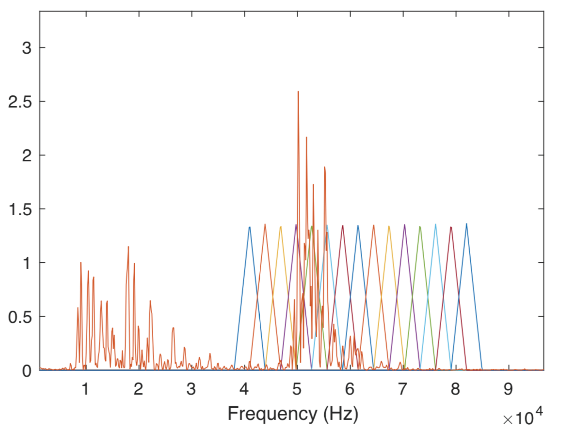
The first stage of the identification consists on the use of a triangular filter bank. The filter bank used in this parameterization is the same as the one used to extract the features of the t-SNE plot to study species separability (Figure 8). The filters that comprise the filter bank are created using a linear scale, which means that all the centers are equally separated. They are triangular in shape, with equal base widths and heights, so their area is unitary. These filters start at the frequency of 38 kHz and end at 80 kHz, which are the start and end frequencies of the calls of the two bat species plus a margin. That way, the frequencies below are not taken into consideration when parameterizing the signal. This is performed to avoid irrelevant noise interference in our analysis. The length of the samples to parameterize has been studied, according to the accuracy of the results obtained in training and testing the classifier. From the study undertaken, presented in Section 4.3, we have selected the 7 ms window. An example of this kind of parameterization is shown in Figure 10. In this figure, a plot of the FFT of the signal and the filters that compose the filter bank are shown. The signal has energy on the frequencies of interest, but also on the lower frequencies. The methodology used only takes into account the higher frequencies.

Both the call pulses and the ambient noise of the audio files are identifiable by their power value in the spectrogram matrices, which reveals the energy of the calls at each time interval and frequency value. The second parameterization technique has followed an image processing approach, using the spectrogram matrices obtained from the analysis of the call fragments starting from 38 kHz frequency and ending at 90 kHz. Their values have been normalized. The Y axis of the matrices corresponds to frequency and its X corresponds to time. As all the sizes are equal, the temporal length used has also been studied to achieve the best performance in the machine learning algorithms. In this case, we have used 20 ms length matrices, after the study described in Section 4.3. An example of a 400 ms length audio file parameterization is shown in Figure 11.

The example of Figure 11, which has five call intervals, has generated four matrices. The fact that one matrix has not been generated is because the distance between the last call and its predecessor was not enough to create two separated matrices that contain only a call. This last call is encircled in purple colour. Both calls would have appeared in the same matrix, so the specifications of the model we wanted to create would have not been accomplished. The last call is discarded and it is not used to train the model.

4.2. Design of the Neural Network Algorithm to Classify the Bat Calls

Several machine learning algorithms were tested for a further comparison of their results and the highest performing ones were selected. Before using the machine learning algorithms, the dataset was balanced, equalizing the number of audio fragments in each of the categories. We used both basic and complex classifiers to find the algorithms that were better adapted to the problem. The basic classifiers used were Random Forest (RF) [50], the Gaussian Naive Bayes (GNB) [51], and Linear Regressors (LR) [52]. Two Neural Networks (NN) were also used: a Feedforward Neural Network (FNN) [53] and a Convolutional Neural Network (CNN) [54]. The performance results obtained demonstrate that simple algorithms achieve higher recall scores but worse precision scores. In the case studied, our concern was to ensure that the prediction outputs were correct, so the metric that we were most interested in were precision or specificity. For that reason, the Neural Networks were chosen as the algorithm to use.

We have used the two different Neural Networks (NNs) that best fit each parameterization of the data. For the filter bank coefficients parameterization, a simple FeedForward Neural Network (FNN) has been used [53]. This kind of network has been elected both for its simplicity and for its good performance with speech recognition [55]. For the energy matrices parameterization, the network used has been a Convolutional Neural Network (CNN). The use of the spectrogram energy matrices gives an image processing approach to the problem and this kind of network achieves high accuracy results in automatic image classification [56].

The models have three categories of data to predict, as they have been trained with the three classes: Pipistrellus pipistrellus, Pipistrellus pygmaeus, and silence. In this stage, in the machine learning algorithms design, the train and validation takes into account three categories, there is no previous selection of bat call against silence, despite the design of the dataset has used this kind of algorithms. The FNN is composed of three dense layers, which define a fully connect each input to each output within its layer. They have a relu activation defined, which transforms any negative input given to zero. It is composed of a first hidden layer with 14 nodes, a second hidden layer with seven nodes, and a final output layer used for regression. The last layer is activated by a softmax function. In both classifiers, the dataset has been split into three categories, which correspond to the training (64%), the validation (16%) and the testing datasets (20%).

Firstly, the training set has been used to fit the model. Each time the model was trained, a test using the validation set was performed to fine-tune its parameters, such as the number of layers that composed the network or the batch size used to train the model. Performance parameters were gathered to avoid overfitting.

The final performance parameters obtained, shown in

Table 1. Results of the classification model using the filter bank coefficients parameterization.

	Pipistrellus pipistrellus	Pipistrellus pygmaeus	Silence
Precision score	64.02%	74.33%	71.48%
Recall score	69.54%	57.41%	81.82%
F1 score	67.43%	66.16%	77.10%

, reflect how different the silence intervals are from the bat calls, as this category is clearly differentiated from the others. On the other hand, bat calls are more likely to be mispredicted. These results coincide with the t-SNE [49] results of the already commented Figure 8.

For the energy matrices, a CNN [54,56] is used. This kind of network is used in computer vision to analyze images and extract their most important and unique aspects that can differentiate them from others. Although our data is not originally an image, the followed analysis procedure is the same. The model is composed of two convolutional layers, whose function is to detect patterns on the matrices received as input. Those layers are configured with eight filters, which define the matrices that slide across each 3 × 3 block of values from the input matrix. We have used two layers, with the first one being responsible for capturing the low-level features and the second the one in charge of perceiving the high-level features. Between the two convolutional layers, a max pooling layer reduces the spatial size of the convolved feature. The computational power to process the data is decreased with dimensionality reduction, extracting the maximum value of each of the obtained matrices. Then, the data are converted into a vector by a flatten layer, and is propagated through a FNN. This NN is composed by two dense layers have 8 and 3 nodes respectively, and the prediction is computed using the softmax classification technique.

Compared with the use of simple FNN, CNNs perform best on capturing local information, such as neighboring pixels in an image and reducing the complexity of the model with the reduction of the number of units in the network by the pooling layer, performing many-to-one mapping. That endows the network with a faster training, the need for fewer samples, and decreases the likelihood of overfitting. The use of a FNN is common in both cases, with the input vector in this case obtained by the flatten operation at the end of the convolutional process. As the parameterization of the data obtained from the filter banks was of the vector type, which is easier to process due to its reduced complexity, it could be directly used as input for the FNN. In this case, the training data have also been split as stated in the previous methodology, with 80% being used for its training and validation and the remaining 20% for testing purposes, using a 5-fold cross-validation principle.

Regarding the obtained performance results (

Table 2. Results of the classification model using the spectrogram energy matrices.

	Pipistrellus pipistrellus	Pipistrellus pygmaeus	Silence
Precision score	71.34%	76.28%	91.31%
Recall score	76.97%	72.10%	89.05%
F1 score	74.05%	74.13%	90.17%

), the results of this model are higher compared to the ones obtained with the FNN. The highest performance enhancement has been on predicting silences, with an enhancement of approximately 15% in the F1 score, from 77.10% to 90.17%. The F1 score of bats [57] has also increased by nearly 10%, achieving in this case F1 score of 74%. These results reveal that the shape of the energy of the pulses in the frequency domain is different, and its study by means of image processing gives good results.

4.3. Study of the Window Length to Use for Parameterizing the Data

For both methodologies, the temporal size of the data for its parameterization has been studied. For its study, the testing files have been split in fragments of fixed length. The studied lengths were estimated by considering the overall duration distribution of the calls. After each of these splittings, a new dataset was created and the obtained data was used to train the prediction model. The length that achieved the best results was the one that was used.

Table 3. Length of the temporal frames with which the data were parameterized and the obtained overall F1 score.

Length of Window (ms)	F1 Score Pipistrellus pipistrellus	F1 Score Pipistrellus pygmaeus	F1 Score Silence
1	57.75%	60.15%	76.60%
3	62.30%	61.62%	76.58%
5	65.38%	64.47%	76.84%
7	67.43%	66.16%	77.10%
9	68.18%	66.69%	76.65%
11	68.09%	68.18%	76.91%
13	68.14%	68.12%	76.94%
15	68.23%	70.97%	78.01%
17	68.63%	69.77%	77.69%
19	69.66%	70.83%	78.75%

presents the overall F1 score [57] obtained for the filter bank coefficients method and

Table 4. Table of the length of the matrices with which the data was parameterized and their overall F1 score.

Length of Generated Matrix (ms)	F1 Score Pipistrellus pipistrellus	F1 Score Pipistrellus pygmaeus
10	61.14%	71.85%
20	78.30%	79.95%
30	79.87%	79.80%
40	79.80%	81.25%
50	81.37%	82.62%
60	78.28%	79.97%
70	61.14%	71.85%

for the spectrogram matrices parameterization. The data contained in the tables are plotted in Figure 12 and Figure 13. To obtain both results, a 5-fold cross-validation has been computed.

In Figure 12, the F1 scores of the different window lengths are drawn. On the one hand, silent fragments do not suffer any severe variation through all the studied window lengths. On the other hand, bat calls do not achieve good prediction results when being parameterized using short window lengths. The low performance when using short frames indicates that the model can not obtain enough information from those data to make accurate predictions. Until the 7 ms window, the bigger the length of the window, the better the performance. Afterwards, results are stabilized, remaining roughly constant although the window expands. From the results obtained, we see that the model’s learning rate decreases after the 7 ms window length. For that reason, it has been decided to select the 7 ms window as the one to use.

In the case of Figure 13, there is a performance improvement at shorter matrices and a deterioration at longer ones. The usage of short matrices does not give enough information to the network to enable it to accurately predict the specie. That could be because the full pulse is not long enough to fit into a short length matrix and just one part of it is analyzed. Contrarily, after 50 ms length, the results of the network decrease, possibly because there is more than one call present in the same matrix, and that generates errors in the estimation of the bat species. The point at which the results stabilize, 20 ms, is the one to be used, as this is the minimal length matrix from which the model can obtain the necessary information to make a reliable prediction.

5. Conclusions and Future Work

There is the possibility of training, validating and testing an algorithm using manually labelled bat calls data capable of identifying the two targeted species, and even the silences in between the calls. This fact encourages the team to keep on working not only using laboratory experiments, but also with real operation experiments in urban environments, where ultrasonic background noise are more common—and so would make bat call identification harder—and the algorithm would have to deal with other species.

From the initial dataset analysis we can conclude that in some cases the two bat species are not easily separable, as they have many common patterns, such as similar frequencies of the calls or their frequency. Splitting the audio files into bat calls and silence fragments provides us with a more precise analysis in the dataset design. As that the studied audio files were split according to the power relation between their peak value and their average value in the first classification, the files have been divided into the ones that present some type of call and the ones that do not. Although this has been a manual and precise task, it has helped to improve the reliability of our dataset, which is published and available for a further analysis [19,20].

Although there is a wide range of features that can be obtained from the audio fragments, those chosen have been designed and implemented to fit with specifications of the problem. The decision to include the pulse bounce to the microphone to the call enables the system to work with more realistic data. If we had not considered this bounce, the system would have got worse results, as it would have had considered the bounce as an independent pulse. The further automatic classification had to be adapted to the data resulting from this parameterization, so two different methodologies were used. The obtained results show a common pattern of both classification models to achieve good results on classifying silent fragments correctly. The analysis of these results show that, surprisingly, these data are better represented by using image processing methods than by being processed by the CNNs. In the future, also a two-stage detection algorithm could be implemented, discarding all analyzed windows corresponding to silences, and using the machine learning algorithms to identify only pieces of data with bat call signal.

Regarding future applications of the developed system, we have to take into consideration that bats are very selective when it comes to the locations they inhabit, so their presence in a particular ecosystem reveals lots of information about both the area’s biological environment and its contribution to the conservation of bat species. They are important bioindicators of some of the most relevant state-of-the-art topics in biology, such as habitat loss and climate change [58]. Their presence in a habitat can also provide a great financial relief for agricultural industries thanks to their contribution as pest managers [2]. Such important values demonstrate the great importance of their monitoring for a better understanding of bats ecology, and as a source of ecological information about a particular habitat. For that reason, the developed approach for an automatic detection and identification of the presence of bats can be applied to many studies of the characteristics of a particular environment.

The quality of the habitat of a city is currently a popular field of study, and in this sense, studies as the one presented in his work can improve the knowledge of the environment in urban areas. One of the aims of the smart cities is to control habitat welfare through the placement of sensors acting as bioindicators. They serve to monitor aspects such as air quality or weather, which are key elements of the global ecosystem. These sensors are responsible for collecting the data to be analyzed and as a source of information for the city acting consequently. The study of the acoustic environment in the cities has been developed in the last years through the deployment of WASNs, and those infrastructures could be a key issue for future evaluations of the biodiversity in cities including the bat population, if properly designed to detect ultrasounds. This preliminary study is just a first approach with two common species of bats in urban habitats and low inference environments, but future studies will improve the accuracy of these sensors, assuming that maybe are part of a bigger monitoring system, and contemplate more wildlife species. The use of sensors to monitor natural bioindicators, such as those animals or plants which are very sensitive to environment conditions, is increasing in popularity. For that reason, one potential application of this project would be to act as a monitoring system of the welfare of the habitat of the city.

References

1. Altringham, J.D. Bats: From Evolution to Conservation; Oxford University Press: Oxford, UK, 2011. [Google Scholar]
2. Cleveland, C.J.; Betke, M.; Federico, P.; Frank, J.D.; Hallam, T.G.; Horn, J.; Lopez, J.D., Jr.; McCracken, G.F.; Medellín, R.A.; Moreno-Valdez, A.; et al. Economic value of the pest control service provided by Brazilian free-tailed bats in south-central Texas. Front. Ecol. Environ. 2006, 4, 238–243. [Google Scholar] [CrossRef]
3. Medellin, R.A.; Gaona, O. Seed Dispersal by Bats and Birds in Forest and Disturbed Habitats of Chiapas, Mexico 1. Biotropica 1999, 31, 478–485. [Google Scholar] [CrossRef]
4. Trejo-Salazar, R.E.; Eguiarte, L.E.; Suro-Piñera, D.; Medellin, R.A. Save our bats, save our tequila: industry and science join forces to help bats and agaves. Nat. Areas J. 2016, 36, 523–531. [Google Scholar] [CrossRef]
5. Russ, J. British Bat Calls: A Guide to Species Identification; Pelagic Publishing: Exeter, UK, 2012. [Google Scholar]
6. Russo, D.; Jones, G. Identification of twenty-two bat species (Mammalia: Chiroptera) from Italy by analysis of time-expanded recordings of echolocation calls. J. Zool. 2002, 258, 91–103. [Google Scholar] [CrossRef]
7. Ahlen, I.; Baagøe, H.J. Use of ultrasound detectors for bat studies in Europe: experiences from field identification, surveys, and monitoring. Acta Chiropterol. 1999, 1, 137–150. [Google Scholar]
8. Vaughan, N.; Jones, G.; Harris, S. Habitat use by bats (Chiroptera) assessed by means of a broad-band acoustic method. J. Appl. Ecol. 1997, 34, 716–730. [Google Scholar] [CrossRef]
9. Walters, C.L.; Freeman, R.; Collen, A.; Dietz, C.; Brock Fenton, M.; Jones, G.; Obrist, M.K.; Puechmaille, S.J.; Sattler, T.; Siemers, B.M.; et al. A continental-scale tool for acoustic identification of E uropean bats. J. Appl. Ecol. 2012, 49, 1064–1074. [Google Scholar] [CrossRef]
10. Russo, D.; Jones, G. Use of foraging habitats by bats in a Mediterranean area determined by acoustic surveys: Conservation implications. Ecography 2003, 26, 197–209. [Google Scholar] [CrossRef]
11. Hayes, J.P. Temporal variation in activity of bats and the design of echolocation-monitoring studies. J. Mammal. 1997, 78, 514–524. [Google Scholar] [CrossRef]
12. Gehrt, S.D.; Chelsvig, J.E. Bat activity in an urban landscape: Patterns at the landscape and microhabitat scale. Ecol. Appl. 2003, 13, 939–950. [Google Scholar] [CrossRef]
13. Gehrt, S.D.; Chelsvig, J.E. Species-specific patterns of bat activity in an urban landscape. Ecol. Appl. 2004, 14, 625–635. [Google Scholar] [CrossRef]
14. Palomo, L.J.; Gisbert, J.; Blanco, J.C. Atlas y Libro Rojo de los Mamíferos Terrestres de España; Organismo Autónomo de Parques Nacionales: Madrid, Spain, 2007. [Google Scholar]
15. Hulva, P.; Horáček, I.; Strelkov, P.P.; Benda, P. Molecular architecture of Pipistrellus pipistrellus/Pipistrellus pygmaeus complex (Chiroptera: Vespertilionidae): Further cryptic species and Mediterranean origin of the divergence. Mol. Phylogenet. Evol. 2004, 32, 1023–1035. [Google Scholar] [CrossRef]
16. Davidson-Watts, I.; Walls, S.; Jones, G. Differential habitat selection by Pipistrellus pipistrellus and Pipistrellus pygmaeus identifies distinct conservation needs for cryptic species of echolocating bats. Biol. Conserv. 2006, 133, 118–127. [Google Scholar] [CrossRef]
17. Obrist, M.K.; Boesch, R.; Flückiger, P.F. Variability in echolocation call design of 26 Swiss bat species: Consequences, limits and options for automated field identification with a synergetic pattern recognition approach. Mammalia 2004, 68, 307–322. [Google Scholar] [CrossRef]
18. Barataud, M. Ecologie Acoustique des Chiroptères d’Europe; Biotope Édition, Mèze; Muséum National dHistoire Naturelle: Paris, France, 2012. [Google Scholar]
19. Russo, D.; Voigt, C.C. The use of automated identification of bat echolocation calls in acoustic monitoring: A cautionary note for a sound analysis. Ecol. Indic. 2016, 66, 598–602. [Google Scholar] [CrossRef]
20. López-Baucells, A.; Torrent, L.; Rocha, R.; Bobrowiec, P.E.; Palmeirim, J.M.; Meyer, C.F. Stronger together: Combining automated classifiers with manual post-validation optimizes the workload vs reliability trade-off of species identification in bat acoustic surveys. Ecol. Inform. 2019, 49, 45–53. [Google Scholar] [CrossRef]
21. Caragliu, A.; Del Bo, C.; Nijkamp, P. Smart cities in Europe. J. Urban Technol. 2011, 18, 65–82. [Google Scholar] [CrossRef]
22. Mermelstein, P. Distance measures for speech recognition, psychological and instrumental. Pattern Recognit. Artif. Intell. 1976, 116, 374–388. [Google Scholar]
23. Mellinger, D.K.; Clark, C.W. Recognizing transient low-frequency whale sounds by spectrogram correlation. J. Acoust. Soc. Am. 2000, 107, 3518–3529. [Google Scholar] [CrossRef]
24. Porter, J.; Arzberger, P.; Braun, H.W.; Bryant, P.; Gage, S.; Hansen, T.; Hanson, P.; Lin, C.C.; Lin, F.P.; Kratz, T.; et al. Wireless sensor networks for ecology. BioScience 2005, 55, 561–572. [Google Scholar] [CrossRef]
25. Boulmaiz, A.; Messadeg, D.; Doghmane, N.; Taleb-Ahmed, A. Robust acoustic bird recognition for habitat monitoring with wireless sensor networks. Int. J. Speech Technol. 2016, 19, 631–645. [Google Scholar] [CrossRef]
26. Wang, H.; Estrin, D.; Girod, L. Preprocessing in a tiered sensor network for habitat monitoring. EURASIP J. Adv. Signal Process. 2003, 2003, 795089. [Google Scholar] [CrossRef]
27. Trifa, V.; Girod, L.; Collier, T.C.; Blumstein, D.; Taylor, C.E. Automated Wildlife Monitoring Using Self-Configuring Sensor Networks Deployed in Natural Habitats; Center for Embedded Network Sensing: Los Angeles, CA, USA, 2007. [Google Scholar]
28. Gros-Desormeaux, H.; Vidot, N.; Hunel, P. Wildlife Assessment Using Wireless Sensor Networks; INTECH Open Access Publisher: Rijeka, Croatia, 2010. [Google Scholar]
29. Stattner, E.; Hunel, P.; Vidot, N.; Collard, M. Acoustic scheme to count bird songs with wireless sensor networks. In Proceedings of the 2011 IEEE International Symposium on a World of Wireless, Mobile and Multimedia Networks (WoWMoM), Lucca, Italy, 20–24 June 2011; pp. 1–3. [Google Scholar]
30. De La Piedra, A.; Braeken, A.; Touhafi, A. Sensor systems based on FPGAs and their applications: A survey. Sensors 2012, 12, 12235–12264. [Google Scholar] [CrossRef]
31. Botteldooren, D.; De Coensel, B.; Oldoni, D.; Van Renterghem, T.; Dauwe, S. Sound monitoring networks new style. In Acoustics 2011: Breaking New Ground: Proceedings of the Annual Conference of the Australian Acoustical Society; Mee, D.J., Hillock, I.D., Eds.; Australian Acoustical Society: Toowong DC, Australia, 2011; pp. 93:1–93:5. [Google Scholar]
32. Mietlicki, F.; Mietlicki, C.; Sineau, M. An innovative approach for long-term environmental noise measurement: RUMEUR network. In Proceedings of the EuroNoise 2015, Maastrich, The Netherlands, 31 May–3 June 2015; EAA-NAG-ABAV: Maastrich, The Netherlands, 2015; pp. 2309–2314. [Google Scholar]
33. Camps-Farrés, J.; Casado-Novas, J. Issues and challenges to improve the Barcelona Noise Monitoring Network. In Proceedings of the EuroNoise 2018, Heraklion, Crete, Greece, 27–31 May 2018; EAA—HELINA: Heraklion, Crete, Greece, 2018; pp. 693–698. [Google Scholar]
34. Bain, M. SENTILO—Sensor and Actuator Platform for Smart Cities. 2014. Available online: https://joinup.ec.europa.eu/document/sentilo-sensor-and-actuator-platform-smart-cities (accessed on 25 June 2018).
35. Bello, J.P.; Silva, C.; Nov, O.; Dubois, R.L.; Arora, A.; Salamon, J.; Mydlarz, C.; Doraiswamy, H. SONYC: A System for Monitoring, Analyzing, and Mitigating Urban Noise Pollution. Commun. ACM 2019, 62, 68–77. [Google Scholar] [CrossRef]
36. Sevillano, X.; Socoró, J.C.; Alías, F.; Bellucci, P.; Peruzzi, L.; Radaelli, S.; Coppi, P.; Nencini, L.; Cerniglia, A.; Bisceglie, A.; et al. DYNAMAP—Development of low cost sensors networks for real time noise mapping. Noise Mapp. 2016, 3, 172–189. [Google Scholar] [CrossRef]
37. Socoró, J.C.; Alías, F.; Alsina-Pagès, R.M. An Anomalous Noise Events Detector for Dynamic Road Traffic Noise Mapping in Real-Life Urban and Suburban Environments. Sensors 2017, 17, 2323. [Google Scholar] [CrossRef] [PubMed]
38. De la Piedra, A.; Benitez-Capistros, F.; Dominguez, F.; Touhafi, A. Wireless sensor networks for environmental research: A survey on limitations and challenges. In Proceedings of the 2013 IEEE EUROCON, Zagreb, Croatia, 1–4 July 2013; pp. 267–274. [Google Scholar] [CrossRef]
39. Rawat, P.; Singh, K.D.; Chaouchi, H.; Bonnin, J.M. Wireless Sensor Networks: A Survey on Recent Developments and Potential Synergies. J. Supercomput. 2014, 68, 1–48. [Google Scholar] [CrossRef]
40. Gillam, E.H.; McCracken, G.F. Variability in the echolocation of Tadarida brasiliensis: Effects of geography and local acoustic environment. Anim. Behav. 2007, 74, 277–286. [Google Scholar] [CrossRef]
41. Echo Meter Touch 2 Handheld Bat Detector from Wildlife Acoustics; Publisher: Wildlife Acoustics. Available online: https://arbtech.co.uk/review-wildlife-acoustics-echo-meter-touch-martin-oconnor/ (accessed on 21 August 2019).
42. Welch, P. The use of fast Fourier transform for the estimation of power spectra: A method based on time averaging over short, modified periodograms. IEEE Trans. Audio Electroacoust. 1967, 15, 70–73. [Google Scholar] [CrossRef] [Green Version]
43. Bergland, G. A guided tour of the fast Fourier transform. IEEE Spectrum 1969, 6, 41–52. [Google Scholar] [CrossRef]
44. Oppenheim, A.V.; Schafer, R.W.; Buck, J.R. Discrete-Time Signal Processing, 2nd ed.; Prentice-Hall, Inc.: Upper Saddle River, NJ, USA, 1999. [Google Scholar]
45. Harris, F.J. On the use of windows for harmonic analysis with the discrete Fourier transform. Proc. IEEE 1978, 66, 51–83. [Google Scholar] [CrossRef]
46. Rydell, J.; Nyman, S.; Eklöf, J.; Jones, G.; Russo, D. Testing the performances of automated identification of bat echolocation calls: A request for prudence. Ecol. Indic. 2017, 78, 416–420. [Google Scholar] [CrossRef] [Green Version]
47. Barataud, M. Acoustic Ecology of European Bats: Species Identification, Study of Their Habitats and Foraging Behaviour, Biotope, éditions ed; Biotope: Méze, France, 2015. [Google Scholar]
48. Brabant, R.; Laurent, Y.; Dolap, U.; Degraer, S.; Poerink, B.J. Comparing the results of four widely used automated bat identification software programs to identify nine bat species in coastal Western Europe. Belg. J. Zool. 2018, 148. [Google Scholar] [CrossRef]
49. Maaten, L.v.d.; Hinton, G. Visualizing data using t-SNE. J. Mach. Learn. Res. 2008, 9, 2579–2605. [Google Scholar]
50. Breiman, L. Random forests. Mach. Learn. 2001, 45, 5–32. [Google Scholar] [CrossRef]
51. Rish, I. An empirical study of the naive Bayes classifier. In IJCAI 2001 Workshop on Empirical Methods in Artificial Intelligence; IJCAI: Seattle, WA, USA, 2001; Volume 3, pp. 41–46. [Google Scholar]
52. Hosmer, D.W., Jr.; Lemeshow, S.; Sturdivant, R.X. Applied Logistic Regression; John Wiley & Sons: Hoboken, NJ, USA, 2013; Volume 398. [Google Scholar]
53. Fine, T.L. Feedforward Neural Network Methodology; Springer Science & Business Media: New York, NY, USA, 2006. [Google Scholar]
54. LeCun, Y.; Bottou, L.; Bengio, Y.; Haffner, P. Gradient-based learning applied to document recognition. Proc. IEEE 1998, 86, 2278–2324. [Google Scholar] [CrossRef] [Green Version]
55. Gevaert, W.; Tsenov, G.; Mladenov, V. Neural networks used for speech recognition. J. Autom. Control 2010, 20, 1–7. [Google Scholar] [CrossRef] [Green Version]
56. Krizhevsky, A.; Sutskever, I.; Hinton, G.E. ImageNet Classification with Deep Convolutional Neural Networks. In Advances in Neural Information Processing Systems 25; Pereira, F., Burges, C.J.C., Bottou, L., Weinberger, K.Q., Eds.; Curran Associates, Inc.: Red Hook, NY, USA, 2012; pp. 1097–1105. [Google Scholar]
57. Rijsbergen, C.J.V. Information Retrieval, 2nd ed.; Butterworth-Heinemann: Newton, MA, USA, 1979. [Google Scholar]
58. Stahlschmidt, P.; Brühl, C.A. Bats as bioindicators—The need of a standardized method for acoustic bat activity surveys. Methods Ecol. Evol. 2012, 3, 503–508. [Google Scholar] [CrossRef]
Figure 1. Pictures of Pipistrellus pipistrellus (left) and Pipistrellus pygmaeus (right).
Applsci 09 03467 g001
Figure 2. Identification of bat call pulses on an sample audio file.
Applsci 09 03467 g002
Figure 3. Echo produced by the bounce of the signal to the microphone.
Applsci 09 03467 g003
Figure 4. Spectrograms of the species. The left hand figures illustrate a close view of the call pulse and the measurement of its bandwidth and duration (85 Power/Frequency). The right hand figures, represents 400 ms’ of an audio fragment containing a bat call.
Applsci 09 03467 g004
Figure 5. Comparison of bat’s call (upper spectrogram) and silence (lower spectrogram). In the upper plot there is a clear differentiation between the bat call pulses and the silence periods between them.
Applsci 09 03467 g005
Figure 6. Diagram of the full process to analyse and segment the initial audio files into the parts that conform the final dataset.
Applsci 09 03467 g006
Figure 7. Total number of audio segments obtained after the initial audio files have been split into the calls and silences, duration, and duration distribution of each bat species and silence.
Applsci 09 03467 g007
Figure 8. t-Distributed Stochastic Neighbor Embedding (t-SNE) plots displaying the separability of the call pulses of the two bat species and with silent intervals added.
Applsci 09 03467 g008
Figure 9. Block diagram of the process used for the automatic classification of the calls contained in an audio file.
Applsci 09 03467 g009
Figure 10. Frequency representation of a sample bat call being filtered with the linear scale triangular filter bank for the coefficients extraction.
Applsci 09 03467 g010
Figure 11. Original spectrogram matrix of a sample audio file and the extracted matrix parameterizations of each call pulse. Each highlighted pulse is associated with the corresponding extracted matrix but the purple one, which does not meet with the parameterization specifications.
Applsci 09 03467 g011
Figure 12. F1 score results of each window length obtained with the filter bank parameterization and the Feedforward Neural Network (FNN).
Applsci 09 03467 g012
Figure 13. F1 score results of each matrix time length obtained with the spectrogram matrices parameterizations a Convolutional Neural Network (CNN).
Applsci 09 03467 g013